

Multiple Systems Estimation: Stratification and Estimation
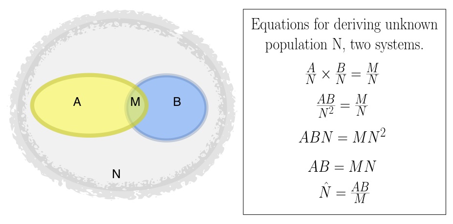
Equations for deriving unknown population N
<< Previous post, MSE: The Matching Process
Q10. What is stratification?
Q11. [In depth] How do HRDAG analysts approach stratification, and why is it important?
Q12. How does MSE find the total number of violations?
Q13. [In depth] What are the assumptions of two-system MSE (capture-recapture)? Why are they not necessary with three or more systems?
Q14. What statistical model(s) does HRDAG typically use to calculate MSE estimates?
In its most general sense, stratification means dividing something up into separate groups, called strata. A group of students may be stratified by grade, households can be stratified by geographic region or income, etc.
Q11. [In depth] How do HRDAG analysts approach stratification, and why is it important?
Stratification, both by definition and for substantive reasons, lowers the variance in capture probabilities, thereby reducing problems with MSE arising from unequal probability of capture. Stratification occurs prior to MSE estimation and (perhaps obviously) requires a separate estimate for each stratum. We stratify estimates on several dimensions, frequently including geography, time, perpetrator, or victim characteristics. For example, our estimates of deaths during Perú’s civil war were stratified by geography and perpetrator group. We conducted separate estimates for several Peruvian departments, as well as separate estimates of violence committed by Peruvian state forces and violence committed by the Shining Path insurgency. By stratifying this way, we were able to control for the fact that lethal violence in some rural areas was much less likely to be reported than lethal violence in urban areas, and lethal violence by Shining Path cadre was much less likely to be reported than lethal violence by state forces. Theoretically, it is possible to stratify on any dimension for which we have complete data. We might perform separate estimates for female and male victims, for violations in the early versus the late years of a conflict, and so on.
Q12. How does MSE find the total number of violations?
MSE estimates the total number of violations by comparing the size of the overlap(s) between lists to the sizes of the lists themselves. If the overlap is small, this implies that the population from which the lists were drawn is much larger than the lists. If, on the other hand, most of the cases on the lists overlap, this implies that the overall population is not much larger than the number of cases listed.
The diagram shows how this works in a simplified way. On the left, list A has 10 individuals, two of whom are also on list B. List B has eight individuals, two of whom are also on list A. We know from probability theory that the probability of being in a random list of size A from a population of size N is A/N. Similarly, the probability of being in a list of size B is B/N, and the probability of being in a list of size M is M/N. We also know that the probability of being in both A and B is the product of the individual probabilities: A/N * B/N. But “A and B” is the same as M, so we can write: A/N * B/N = M/N. From there, we can solve the equation for the unknown total population size, N: N = A*B/M.
Lists A and B are the same size on both left and right (A=10, B=8). However, on the left, A and B overlap only a little, while on the right, A and B overlap very significantly (i.e., M is large compared to A and B). As expected, when we plug A, B and M into the equation above, we find that N (the overall population) is much larger when the overlap is small than when it is large.
Remember that this is a simplified example. While the intuition behind MSE follows the two-list case closely, the two-list case relies on some assumptions about the lists that human rights data typically cannot meet. However, when we expand to three or more lists, these assumptions no longer apply, because we can use more complex statistics than those in the equation above. Generally, when we talk about MSE, we are talking about applying these more complex methods, which are described below.
Q13. [In depth] What are the assumptions of two-system MSE (capture-recapture)? Why are they not necessary with three or more systems?
Two-system capture-recapture analysis depends on four assumptions about the lists and the population from which they are drawn. First, the closed system assumption means that the population does not change during measurement. Second, we assume that the overlap between datasets is correctly identified, i.e., we assume perfect matching. Third, the dual-system estimator assumes equal probability of capture for all individuals. Fourth and finally, the dual-system estimator assumes that the lists are independent, i.e., that probability of capture in one list does not affect probability of capture in the other. In the table below, we review these assumptions, discuss whether each assumption changes when three or more systems are used, and list synonyms for violation of the assumption that are frequently seen in academic discussions of MSE and related techniques.
|
2-System Assumption |
Can be modeled with 3+ systems? |
Other terms for violation of assumption |
| Closed system: The population of interest does not change during the measurement period. | Models exist for ‘open systems’ which allow for changes to the population during the period of study. However, the closed system assumption holds for lethal violence: if we are collecting reports in 2012 about deaths in 2010, there can be no new events in 2010. | |
| Perfect matching: The overlap between systems (i.e., the group of cases recorded in more than one list) is perfectly identified. | No. | |
| Equal probability of capture: For every data system, each individual has an equal probability of being captured. For example, every death has probability X of being recorded in list 1, every death has probability Y of being recorded in list 2, and so on. | Yes. Can stratify or model directly. | “unequal catchability,” “unit heterogeneity,” “unequal probability of capture,” “capture heterogeneity” |
| Independence of lists: Capture in one list does not affect probability of capture in another list. For example, being reported to one NGO does not change the probability that an individual is reported to another. | Yes. Can model directly. | “list dependence,” “correlated lists” |
As the table above suggests, the two final assumptions—equal catchability and list independence—are unnecessary for MSE analyses with >=3 datasets, because both individual differences in catchability and dependence between lists can be parameterized and modeled. However, it is important to note that it is not always practically feasible to model both capture probability and list dependences.
Q14. What statistical model(s) does HRDAG typically use to calculate MSE estimates?
Our estimates are primarily based on Poisson regression. As we describe the model, for convenience’s sake, let’s say we’re dealing with three lists: 1, 2, and 3. Let’s further say that the number of violent incidents selected into a list or combination of lists is m100, m010, m001, m110, m101, m011, and m111. Each of these cells is a count of cases. For example, m100 is the number of cases in only list 1; m110 is the number of cases that appear in lists 1 and 2, but not list 3—and so on. The m‘s are called cell counts (as in a contingency table), and Poisson regression treats these cell counts—not the underlying individual cases—as data. The (log of the) expected cell count m000 is a function of the other observed cell counts, as shown in the equation below.
log(m000) = a + β1(m100) + β2(m010) + β3(m001) + β12(m110) + β13(m101) + β23(m011)
This is the saturated form of the log-linear models introduced in Bishop, Fienberg and Holland (1975 [2007 revised edition]). When estimation of the total “population” of violent incidents is the goal (as it typically is with MSE), the key value here is the intercept a. To estimate log(m000), all the other m values are zero. Therefore the only term that contributes to the estimate of log(m000) is a. The value of m000 is therefore the exponentiated value of a, that is, ea. The total number of cases is the sum of the observed cases (that is, the seven values of m) plus ea.
As with any regression and data mining model, we want to avoid overfitting. That is, we wish to balance our interest in goodness of fit with our interest in simple, parsimonious models. We need to find the best model in order to get an accurate estimate of a. Thus, we should determine whether the full model above, which assumes that all three two-way interactions between datasets are important, is actually necessary. There are three simpler models that assume only one two-way interaction—
log(m000) = a + β1(m100) + β2(m010) + β3(m001) + β12(m110)
log(m000) = a + β1(m100) + β2(m010) + β3(m001) + β13(m101)
log(m000) = a + β1(m100) + β2(m010) + β3(m001) + β23(m011)
—as well as three models that assume exactly two two-way interactions—
log(m000) = a + β1(m100) + β2(m010) + β3(m001) + β12(m110) + β13(m101)
log(m000) = a + β1(m100) + β2(m010) + β3(m001) + β12(m110) + β23(m011)
log(m000) = a + β1(m100) + β2(m010) + β3(m001) + β13(m101) + β23(m011)
Because there are just seven possible models, when we model selection into three datasets, we estimate all seven of these, and choose the model that minimizes the Bayesian Information Criterion (BIC), a test that weighs goodness of fit against degrees of freedom. With four or more systems, estimating all possible models in order to directly compare BIC is infeasible; instead, we use a branch-and-bound algorithm (see descriptions here, here, and here), as implemented in the R package BMA. (Note that the implementation of branch-and-bound used in package BMA is the R package leaps.)
We then use the R package Rcapture, designed specifically for multiple-recapture estimations, to produce estimates and confidence intervals. (Confidence intervals in Rcapture are computed using the profile loglikelihood method introduced by Cormack; see this 2007 article by Baillargeon and Rivest, at page 7.)
In some earlier projects, we used alternate methods of model selection and variance estimation. For example, in our estimation of deaths in Perú, we selected models by minimizing the ratio of the chi-square statistic to the degrees of freedom (after first discarding models with unacceptable chi-square values). In many pre-2010 projects, we used jackknifing to arrive at variance estimates. And, in a 2007 estimation of disappearances in Casanare, Colombia, we used Bayesian Model Averaging to more fully incorporate model uncertainty into our estimates. Despite these variations, however, our MSE analyses have three things in common: they use log-linear modeling to estimate the number of uncounted cases; model selection depends on the balance between goodness of fit and parsimony; and they employ variance estimators appropriate to the data.
Stay tuned for the next and final MSE post, Does It Really Work? >>
[Creative Commons BY-NC-SA, excluding image]