
Teaching a small classifier to spend expensive attention wisely
17 August 2026
Written by:
Stephanie Andrews, Research Fellow at the Global Rights Innovation Lab Clinic
A division of labor between large language models, human reviewers, and a one-megabyte classifier, on a corpus of police misconduct files.
The needle and the haystack
When a California law enforcement agency opens an internal investigation into one of its officers, it is required to tell that officer in writing. The document that does this – a notice of complaint addressed directly to the subject of the investigation – is one of the most useful pages in a misconduct file. It dates the start of the investigation, names the original allegations, and identifies the officer as the person under scrutiny rather than a witness, a complainant, or a supervisor in the chain of command. For a researcher reconstructing what happened in a case, it is one of the first things to look for.
The trouble is finding it. The Community Law Enforcement Accountability Network (CLEAN) initiative works with millions of pages of records released under California's police transparency laws. Unfortunately, those pages do not arrive as tidy, one-document-per-file PDFs. A single file is often a stack of concatenated documents: reports, complaints, interview transcripts, and administrative memos scanned together, with the notice of complaint buried somewhere inside. The notices also are not uniform: their layout varies from agency to agency, with no single template to match against. The task is not "which files contain a notice" but the finer-grained "which page is the first page of a subject notice."
We could try to read everything, but the corpus is far too large for exhaustive human review. We could ask a large language model about every page, but at millions of pages that is prohibitively expensive and slow. So from the start the real question was not whether to use LLMs, but where to spend them, and where to spend the even scarcer resource: human attention.
The idea: a small routing model built from LLM labels and human ground truth
The way to spend that attention well is to not spend it on every page. A trained classifier can read every page instead. The problem is simple enough because each page is a binary yes-or-no question, and the notices share enough common language for a bespoke classifier to learn from. So we built one in a teacher-student setup: two LLM teachers produce labels, and a small student model learns from them to become a cheap classifier you could deploy.
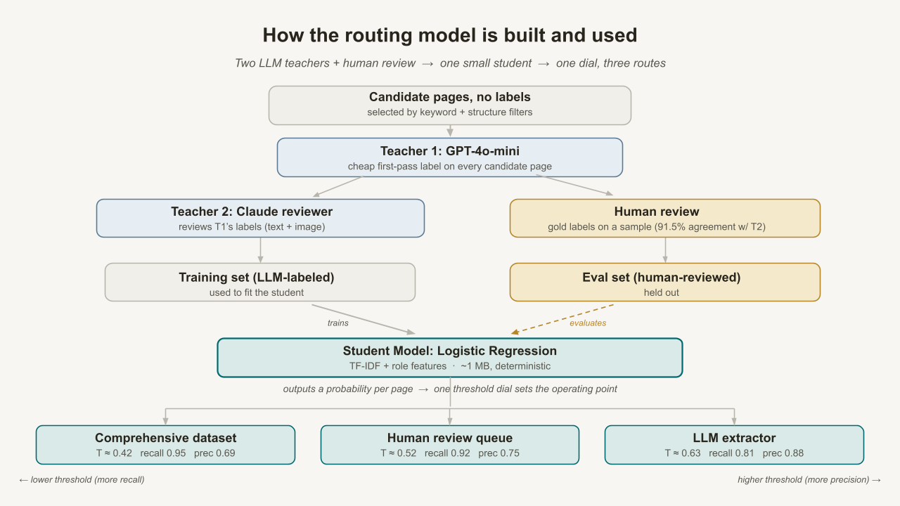
Figure 1. Pipeline architecture. Two LLM teachers and a human reviewer produce labels; a cheap student distills them. The trained student then routes pages to one of three downstream consumers via threshold tuning.
The two teachers are both large language models, serving different but complementary purposes:
- A first-pass LLM labeler (GPT-4o-mini, reading text only) has the most throughput and the least authority. It is a small and relatively inexpensive model, used here to produce cheap candidates rather than definitive classifications.
- A second LLM acting as a reviewer (Claude Sonnet 4.6, reading both text and image) has more authority and still far more throughput than a person. It is a larger and more capable model, used to review each first-pass label against the page itself.
Human review sits outside this teacher-student loop. It is the scarce, highest-authority signal that corrects the LLMs where it can and provides the held-out gold set used to evaluate the final model.
From the LLM labels we distill a student model that runs entirely on our own machines and fits in a one-megabyte file. The distillation process here is simple: the teachers each give a discrete verdict (yes, no, or "ambiguous"), and the student learns from those hard labels.
After the student is trained, its role inverts. The classifier stops being the model the teachers label for and becomes the router that decides where the scarce resources – human review and downstream LLM calls – get spent. That is the idea this post is built on: creating small models that can direct expensive attention, human or model, where it is most needed. The sections that follow walk through how we built it.
Finding candidates without labels
We first needed a way to choose which pages are worth labeling. Random sampling would be wasteful; subject notices are rare in the raw corpus, so a random draw is mostly low-signal pages. Instead, we scored every page with a small set of lexical patterns that tend to co-occur with investigation notices: the word notice, the word complaint, internal affairs or professional standards, the phrase this is to inform you, and the structural markers of a memo header (TO:, FROM: <rank>, SUBJECT:).
HIT_PATTERNS = {
    "hit_notice":        r"\bnotice\b",
    "hit_complaint":     r"\bcomplaint\b",
    "hit_investigation": r"\binvestigat(?:ion|ive)\b",
    "hit_admin":         r"administrative\s+investigation|admin(?:\.|istrative)?\s+inv",
    "hit_ia":            r"internal affairs|professional standards",
    "hit_inform":        r"this is to inform you",
    "hit_to":            r"(?m)^\s*to:\s+.+",
    "hit_from":          r"(?m)^\s*from:\s+(?:sergeant|sgt\.?|lieutenant|lt\.?|captain|chief|commander)\b",
    "hit_subject":       r"(?m)^\s*subject:\s+.+",
}
A page's score is the number of patterns it matches. We used these scores to bin pages into high, medium, and low tiers and sampled across all three, drawing more heavily from the high-signal tier where positives are likeliest. This score was only a sampling heuristic; the classifier never saw it. It was used solely to decide which pages we sampled, not how they're labeled.
While the tiers balance for signal, we also needed to balance for geography. Subject notices are formatted differently from county to county, so a set dominated by a few heavily documented departments would teach the model one county's template instead of the general pattern. To address that, we capped how many pages any one county contributed (a handful of likely-subject pages and a few more likely-negatives each) and topped up from the global pool to hit the target size.
Teacher 1: cheap first-pass labels
We then labelled in two passes: a cheap, high-volume first pass followed by a more authoritative review. For the first labelling pass we used GPT-4o-mini, prompted to read a single page's extracted text and decide whether it is the first page of a notice sent to the subject of the investigation. The prompt enumerated the conditions that must all hold and defaults to OTHER whenever anything is unclear.
A page is SUBJECT_NOTICE_FIRST_PAGE ONLY if ALL of the following are true:
  - It is clearly addressed TO the officer (e.g., "TO: Officer John Smith").
  - The memo informs THEM that THEY are the subject of an internal/administrative investigation.
  - It explicitly states or strongly implies misconduct allegations involving THEM.
  - It usually describes rights/procedures (POBR rights, representation, interview scheduling).
  - It is the FIRST page (greeting/header/subject line appears on this page).
...
Be conservative: if ANY requirement is unclear or missing, choose OTHER.
Human review
Because GPT's labels were only a starting point, we checked a subset of them by hand. To make that fast, we wrote a small command-line review tool that printed one page at a time with GPT's call and reason, showed the OCR text, and asked a human reviewer for a one-key verdict.
[ 23/462 ]
SHA: 4f1a... Page: 1
Agency: ...    County: ...
GPT label: SUBJECT_NOTICE_FIRST_PAGE    (conf=0.71)
GPT reason: addressed to the officer; references an internal investigation
--------------------------------------------------------------------------------
OCR TEXT:
  TO: Officer ...   RE: Notice of Administrative Investigation ...
--------------------------------------------------------------------------------
Your options:
  [Y] yes, GPT label is correct
  [N] no, GPT label is NOT correct
  [M] maybe / unclear
  [S] skip   [Q] quit and save
A Y kept GPT's label, an N flipped it, and an M marked the page ambiguous. Each verdict was then written back to a reviewed_label column for the corresponding page. Across the reviewed pages, GPT's labels were roughly 88% correct, 7% wrong, and 5% ambiguous.
These human verdicts informed both training and evaluation. For training, they overrode the LLM labels on any page a person has reviewed. For evaluation, a separate slice of human-reviewed pages was held out as the gold set, used only to test the finished model.
This process was essential but limited by throughput. Reading a page carefully takes minutes. Human review produces the highest-quality labels but the fewest of them, far too few to label the corpus on their own.
Teacher 2: an LLM reviewer
So we added a second teacher, Claude Sonnet 4.6, to do what people could not at volume. This LLM served as a reviewer and was given both the OCR text and the rendered image of the page. Text alone throws away the cues that separate a subject notice from a look-alike: the layout of an address block, a redaction bar, whether a name is the original recipient or only CC'd. The image provided those cues. With those cues visible, the LLM reviewer could decide with the same information a human would have. The LLM reviewer then returned the same yes/no/ambiguous verdicts a human reviewer does, so its labels slot into the training set the same way.
Before we let the LLM reviewer’s labels into the training set, we had to answer an obvious question: are they good enough to stand in for a human? We checked by comparing its determinations against our set of human-reviewed determinations on the pages both had judged. Across roughly 460 shared pages where both gave a clear yes-or-no call, the LLM reviewer and human reviewers agreed about 91.5% of the time.
Through error analysis we determined that these disagreements were not random noise. The LLM reviewer leaned toward calling a borderline page a subject notice more often than humans do, over-flagging toward the positive class by a factor of about three on the boundary cases. However, those cases were genuine definitional edges (interview-notification memos, administrative orders to surrender equipment, notices of discipline), the same pages where human reviewers might hesitate. We ultimately did not correct for this, instead noting it as a known bias in the LLM-reviewed pages.
We then combined the reviewed labels into one training set, keeping the most authoritative label for each page: a human verdict where we have one, otherwise using the LLM’s. Every label in the set has been checked by a human or by the LLM reviewer; GPT's first pass only nominated the candidates that those reviews then confirmed or overturned.
Building the student: features
The reviewed labels gave us a merged training set of 1,648 labeled pages, 291 of them subject notices.[1] The student model then came together through three choices: how to turn each page into features, which engineered features to add on top, and which model family to train on them. This section covers the first two choices; the next compares model families and picks one.
Our first model was a simple baseline: TF-IDF[2] over the page text fed to a logistic regression[3]. We tested that representation against sentence embeddings and found the distinguishing information was lexical, not semantic. A subject notice and a witness notice can mean almost the same thing while differing in a few specific phrasings. Embeddings, which compress meaning, blurred exactly the distinction we needed; TF-IDF beat embeddings on every classifier and every setting we tried.
But that plain TF-IDF baseline still made a common error. It confused witness notices with subject notices. This was unsurprising since the two have very similar memo layouts and overlapping vocabulary. What separates them most is the role the page assigns to its reader. A subject notice says "you are the subject of an investigation"; a witness notice says "you are a witness."
A bag of words and bigrams cannot represent that relationship because it has no notion of which words modify which. So we added it explicitly. Five engineered features encoded the attribution: whether "you" appears near "subject," whether "you" appears near "witness," and so on.
ROLE_FEATURE_NAMES = [
    "role_you_subj",       # "you are/were/have been [the/a] subject"
    "role_you_wit",        # same, but "witness"
    "role_you_not_wit",    # "you are/were not [a] witness"
    "role_prox_you_subj",  # a "you"-token with a "subject"-token within +/-5 positions
    "role_prox_you_wit",   # same proximity count for "witness"
]

def role_proximity_features(text, window=5):
    tokens = re.findall(r"\w+", text.lower())
    return np.array([
        len(_PATTERN_YOU_SUBJ.findall(text)) + len(_PATTERN_AS_SUBJ.findall(text)),
        len(_PATTERN_YOU_WIT.findall(text))  + len(_PATTERN_AS_WIT.findall(text)),
        len(_PATTERN_YOU_NOT_WIT.findall(text)),
        _prox_count(tokens, _YOU_TOKENS, "subject", window),
        _prox_count(tokens, _YOU_TOKENS, "witness", window),
    ], dtype=np.float64)
We confirmed these features later, once we had chosen a classifier. In the final model (logistic regression), the "you are the subject" feature has a weight of +1.531, roughly five times the model's mean absolute coefficient of 0.32. The "you are a witness" feature has a weight of −1.267. One feature checks for "you are not a witness," a phrasing that does not actually occur in these documents. Its weight is exactly 0.000, as we predicted.
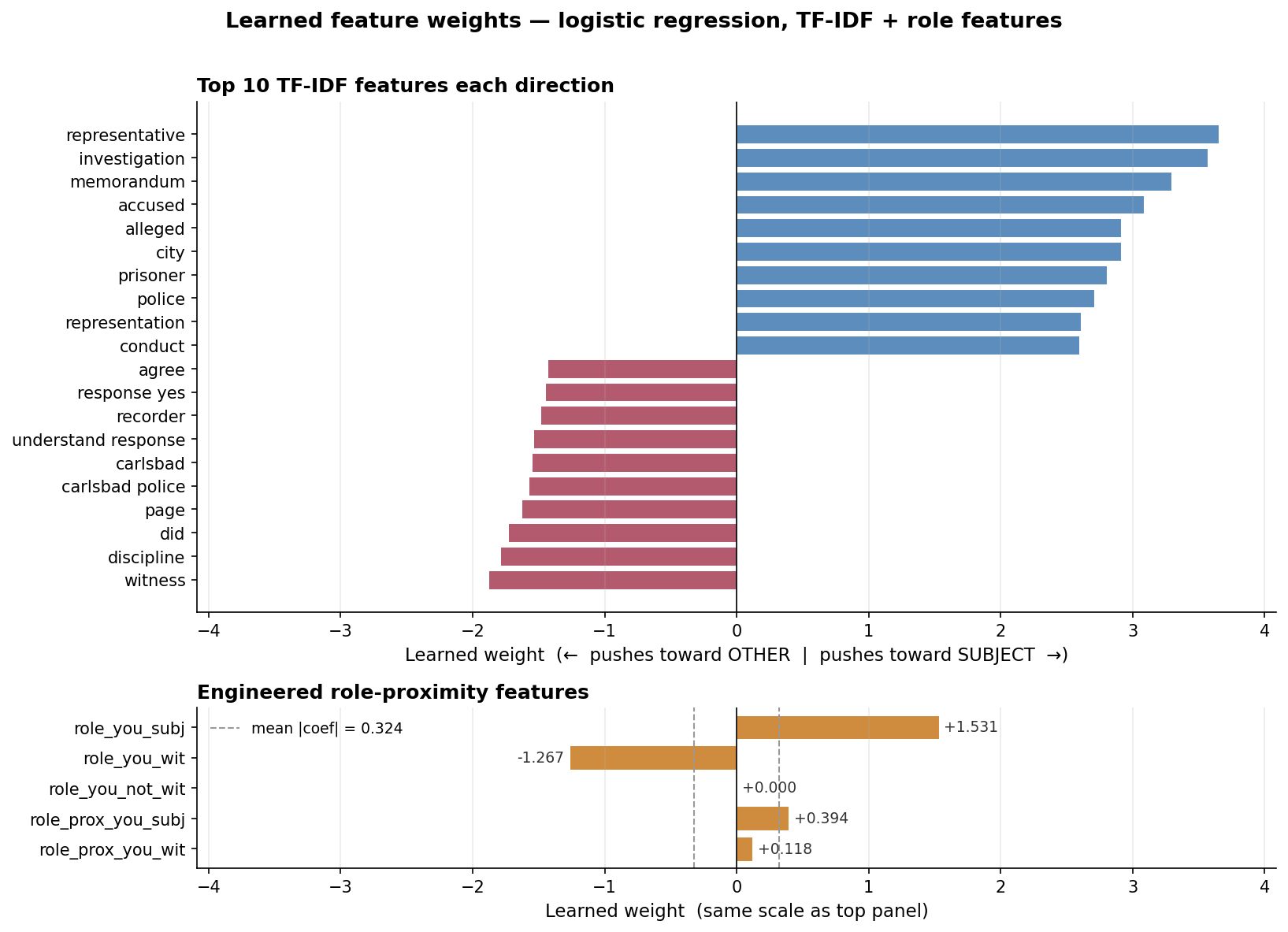
Figure 2. The 10 strongest TF-IDF features in each direction (top), and the engineered role-proximity features on the same scale (bottom). Dashed lines mark ±the mean absolute coefficient; the strongest role features sit several times beyond it.
Together, the TF-IDF text and these five role features made up the feature set we trained on.
Choosing the classifier
The role features helped most, but the choice of classifier was its own question. We compared four model families: logistic regression, linear SVM (Support Vector Machine), random forest, and gradient boosting. For the two with a regularization parameter (logistic regression and a calibrated linear SVM), we tuned C[4] by testing a range of values on each representation. Sentence embeddings underperformed TF-IDF across every setting, so we kept TF-IDF plus role features. Random forest and gradient boosting used fixed settings (300 trees with class-balanced weights for RF; 200 stages for GBM) selected from a small set of tested configurations.
Every figure in the table below is for the subject-notice class, the positive class we care about; the full per-class metrics are in the appendix. Recall[5] is the share of true subject notices the model catches; precision[6] is the share of its positive calls that are actually correct. The two trade off against each other as the decision threshold moves. F1 is their harmonic mean at the default 0.5 threshold, and average precision (AP) is the area under the whole precision-recall curve, a single threshold-independent score. We compared the models mainly on recall, while requiring precision to stay usable.
The cross-validated[7] results for the subject-notice class were as follows:
| Model (TF-IDF + roles) | Recall @0.5 | Precision @0.5 | F1 @0.5 | AP |
|---|---|---|---|---|
| Logistic regression, C=5 | 0.849 | 0.746 | 0.794 | 0.882 |
| Gradient boosting (200 stages) | 0.715 | 0.867 | 0.783 | 0.885 |
| Random forest (300 trees) | 0.677 | 0.908 | 0.776 | 0.882 |
| Linear SVM, C=0.1 (calibrated) | 0.639 | 0.721 | 0.678 | 0.810 |
Two things stood out. First, the tree-based models bought precision by giving up recall: the random forest model had 0.908 precision but caught only about two-thirds of the subject notices, the wrong trade for a task where a missed notice is an overlooked document. Second, logistic regression, random forest, and gradient boosting landed within a point or two of each other on average precision (around 0.88); average precision alone did not separate them.
So we chose logistic regression. It gave the best recall at usable precision, and unlike the tree models, its per-feature weights were directly readable.
Fitting and evaluating the final model
With the classifier chosen, we next fit and bundled the model and its featurizer into a small, self-contained file.
clf_params = {"C": 5.0, "class_weight": "balanced",
              "solver": "liblinear", "max_iter": 1000, "random_state": 24}
clf = make_classifier("logistic_regression", clf_params)
clf.fit(X_train, train_df["final_label"])

bundle = ModelBundle(classifier=clf, featurizer=TfidfWithRoles(tfidf))
save_model(bundle, model_dir, name="tfidf_roles_logreg_c5")
We then evaluated the model two ways.
The first was five-fold stratified cross-validation over the full 1,648-page training set. Split the data into five folds, train on four, test on the fifth, rotate, and average. With TF-IDF plus the role features and logistic regression, recall was 0.849 ± 0.028 with precision around 0.75.
This first measure had a limit: many of the pages were labeled by an LLM reviewer, so it partly reflected how well the model matched that reviewer rather than the truth.
The second evaluation used a different split to address that. Cross-validation compared architectures and hyperparameters on rotating folds of the full labeled set, gold pages included. This second protocol held them out: we retrained only on the LLM-labeled pages (1,186) and tested on the 462 pages a human reviewer had confirmed, the gold eval set. No gold-set page appeared in training so every test label was one the final model never saw.
On that gold set, the subject-notice class had recall 0.927 and precision 0.727. The model found almost every subject notice but flagged some other pages as notices too. The other class was the mirror image, with precision 0.975 and recall 0.892.[8] These results were from using the model's default threshold of 0.5.[9] Average precision, the area under the precision-recall curve across all thresholds, was 0.911 for the subject class on the gold set, slightly above the 0.882 from cross-validation. This suggests the model generalizes to human-confirmed labels it never trained on.
The two evaluations were not redundant: cross-validation shows how the model performs on data like its training data, and the human-reviewed holdout shows it is not merely echoing the LLM reviewer.
One model, one dial: routing to humans and to LLMs
The final model was trained once, and a single dial – its decision threshold – enables tuning its behavior afterward. For each page the classifier returns a score between 0 and 1, which is the probability that the page is a subject notice. The threshold is the cutoff we apply to that score: pages at or above it are called subject notices, pages below are called other. Moving the cutoff up or down slides the model along its precision-recall curve, letting the same small classifier serve very different downstream consumers without retraining.
bundle = joblib.load("models/tfidf_roles_logreg_c5.joblib")
X = bundle.featurizer.transform(pages["text"])
pos = list(bundle.classifier.classes_).index("SUBJECT_NOTICE_FIRST_PAGE")
scores = bundle.classifier.predict_proba(X)[:, pos]   # e.g. 0.02, 0.36, 0.92, 0.996
The figure below plots the model's subject-notice precision, recall, and F1 on the gold set as the threshold sweeps from 0 to 1. The three marked points are example operating points, one per row of the table that follows.
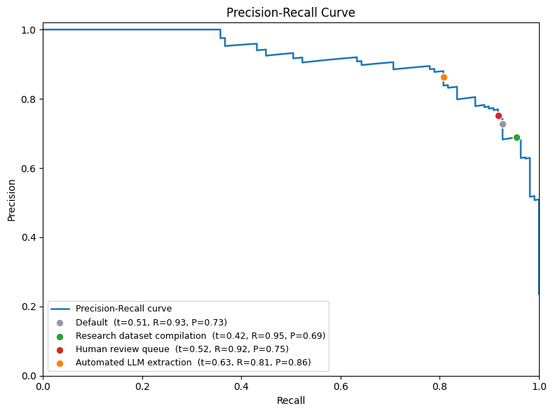
Figure 3. PR curve on the gold set (AP=0.911), with three deployment operating points marked. The same trained model can serve different downstream consumers by sliding the decision threshold: low threshold for comprehensive dataset compilation, a middle threshold for a human review queue, and a higher threshold for automated LLM extraction where API cost favors precision.
| Downstream consumer | What's scarce | Optimize for | Threshold | Recall | Precision |
|---|---|---|---|---|---|
| Human review queue | reviewer time | recall | ~0.52 | 0.917 | 0.752 |
| Automated LLM extraction | API cost | precision | ~0.63 | 0.807 | 0.880 |
| Comprehensive dataset | completeness | maximum recall | ~0.42 | 0.954 | 0.689 |
That threshold is how we match the classifier’s behavior to the cost of whoever, or whatever, looks next. For a human review queue, we favor recall and accept the extra false positives, because a person can dismiss a wrong page in a second while a missed page is a document lost from the record. For an LLM extractor – a downstream model that pulls structured fields out of each page – we favor precision, because every page forwarded costs an API call. For building a comprehensive research-grade dataset that a human will later pass over in full, we push the threshold as low as it goes to maximize recall and let the later human pass clean up.
But the score is useful on its own too, not just as input to a threshold. Thresholding collapses each page's score into a single classification, but the score itself carries more information than that. A downstream consumer can also act on it directly to:
- Order a review queue. Reviewers don't have to take pages in document order. Sorting by score puts the most-likely notices first. If the queue gets truncated for time, it loses its least-certain items rather than random ones.
- Carve out a confident tail and skip review entirely. On the gold set, every page scoring below ~0.1 was a true negative, and pages above ~0.9 were right ~96% of the time. Those two tails are also where most of the corpus lives: across the full corpus of ~2.8 million pages, 91.4% (~2.6 M pages) score below 0.1 and less than 0.1% (~1,600 pages) score above 0.9, leaving roughly 8.5% (~241,000 pages) in the uncertain middle. A pipeline can auto-accept the high tail, auto-reject the low tail, and spend its scarce human or LLM attention on that middle band.
- Pass the score along as context. When the next stage is an LLM extractor, the score can be sent with the page ("the upstream classifier rated this 0.93"). The extractor, or a person reading its output, then knows whether it is looking at a near-certain notice or a borderline call.
One caveat on reading the score. Because the model is trained with balanced class weights (which push minority-class scores up to favor recall), the outputs are well-ordered ranking scores rather than calibrated probabilities. At the extremes they track reality closely (a 0.02 is almost certainly not a notice; a 0.95 almost certainly is), but in the uncertain middle they run optimistic: a page scored 0.44 was a true notice closer to one time in five than the number suggests. The ordering is what thresholds and queues depend on, so this is fine for routing, but a system that wants to read the score as a true probability would need a calibration step first.
Approaches that didn't improve the model
We tested two other approaches we thought were promising: a fine-tuned transformer and an ensemble. Neither improved on the baseline model, but both failures were informative.
The first was a contextual language model (DistilBERT) fine-tuned on the training set. Its mean recall was about the same as the baseline model's but it was much less stable across folds (two to three times the variance). The likely reason is data volume: 1,600 examples with class imbalance may be enough for a well-tuned linear model but could leave a transformer with too little to reliably converge.
The second was ensembling. A soft-vote ensemble combining the linear model with a random forest scored higher in cross-validation, but that gain disappeared when evaluating on the human-reviewed gold set. The ensemble model had picked up the teacher's labeling quirks, and the trees’ flexibility likely let them fit those quirks more tightly.
On a training set this small, the two more expressive alternatives we tested didn't help. One gave inconsistent results across folds (DistilBERT); the other overfit to the teacher's idiosyncrasies (the ensemble model).
Limits and what comes next
This process comes with several limitations. The most important is how to interpret the results. Our pages were chosen through stratified sampling, not at random from the corpus, so they describe the model's behavior on our labeled distribution rather than a corpus-wide estimate. The rest are properties of the system itself: it depends on OCR quality, a few features overfit to specific agencies and names, and the distillation uses hard labels rather than soft ones.
Some precision errors also came from the model recognizing notice content on pages that are not the first page of a notice. For that, others on the CLEAN team have built a page-stream segmentation (PSS) pipeline that identifies document boundaries within a PDF. Passing only PSS-identified first pages to the classifier should reduce these errors. And finally, the amount of labeled data is itself a major limitation: even a fine-tuned DistilBERT model did not beat a linear baseline model at this scale, which points to data volume as a potential bottleneck. One next step to try is providing more labelled data behind these and other models.
This approach comes down to a small model deciding where expensive attention goes. Our small classifier does not replace the large language models or the human reviewers in this pipeline. It is instead the cheap, auditable front door that can route both kinds of expensive attention. Train it once then slide its threshold; the same model fills a human review queue or feeds a downstream LLM. The classifier decides who looks. The people, and sometimes the models, decide what is true.
Appendix: full per-class metrics
The tables above focus on the subject-notice class as it is the class the pipeline exists to find. The final model's per-class metrics on the held-out gold set are below.
| Class | Recall | Precision | F1 |
|---|---|---|---|
| Subject notice | 0.927 | 0.727 | 0.815 |
| Other | 0.892 | 0.975 | 0.932 |
Overall accuracy on the gold set is 0.900. The subject-class average precision is 0.911. Across both classes, the macro average is precision 0.851 and recall 0.909. The support-weighted average is precision 0.917 and recall 0.900.
Acknowledgements
This was produced by the Global Rights Innovation Lab (GRIL) clinic, which makes improvements to and surfaces insights from the Police Records Access Project to support the work of HRDAG and the Community Law Enforcement Accountability Network (CLEAN).
[1] Every number comes from the 1,648 labeled pages (291 subject notices, 1,357 other). Cross-validation uses all 1,648 with rotating folds. Final gold-set numbers train on 1,186 pages and test on 462 human-reviewed pages held out as the gold set. Every model uses the same fixed random seed.
[2] TF-IDF (term frequency–inverse document frequency) turns each page into a vector of word and word-pair counts, then down-weights words that appear in almost every page (so common terms like "the" or "officer" count for little) and up-weights words that are distinctive to a page. It is a classic, fully transparent text representation: every dimension is a literal word or bigram you can read off.
[3] Logistic regression is a linear classifier: it learns one weight per feature, sums the weighted feature values for a page, and squashes the total into a score between 0 and 1. Because each feature has a single readable weight, you can inspect exactly why it made a call, which is how we confirmed the role features were doing their job.
[4] C controls how closely the model fits its training data; smaller C means stronger regularization. We swept C values for each model and representation. For logistic regression the best C rose as the labeled set grew, from 0.05 on the early data to 5 on the full set, since more data lets the model fit more closely without overfitting; the linear SVM's best C was 0.1.
[5] Recall = true positives ÷ all actual positives. "Of the subject notices that really exist in the set, what fraction did the model find?" High recall means few misses.
[6] Precision = true positives ÷ all predicted positives. "Of the pages the model flagged as subject notices, what fraction really are?" High precision means few false alarms.
[7] Cross-validation splits the labeled data into k equal folds (here k = 5), trains on k−1 of them and tests on the held-out fold, then rotates so every fold is tested once. Averaging the five scores gives a more stable estimate than a single train/test split, and the spread across folds is itself informative about stability.
[8] We report the two classes separately rather than a single averaged score. The macro average (precision 0.851, recall 0.909) and the support-weighted average (precision 0.917, recall 0.900) are available but less informative here: the per-class numbers, and the errors the model makes, are what tell us most how the model will behave downstream.
[9] The model emits a probability per page between 0 and 1; the threshold is the cutoff above which a page is labeled a subject notice. The default of 0.5 is a convention that can be adjusted to favor recall or precision. The next section tunes that threshold up or down depending on who is downstream.